
【翻译】第三十四篇 Rediscover an underused probability distribution method
本帖最后由 小编D 于 2011-12-15 17:58 编辑 _
你好,我是小编H。请对以下文章有翻译兴趣的组员留下你的预计完成时间,并发短信息联系小编H,以便小编登记翻译者信息以及文章最终完成时的奖惩工作。感谢支持翻译组!
by Lynne B. Hare
The Poisson distribution (pronounced "pwas-son" where the n is spoken through the nose—don’t ask) may be the Rodney Dangerfield of statistics. It doesn’t get the use—and respect—it deserves. Yet, when applied properly, it can aid the decision-making process considerably.
Here are two examples of its application in the real world. Given these, perhaps you can think of more applications in your own line of work.
Needles in haystacks
For want of preventive maintenance, a screen broke off its frame, disintegrated, mixed with a key product ingredient and then mixed with the finished product. "We think we got it all," said the quality manager. "We ran the finished product over magnets, and we’ve captured enough pieces to reproduce almost an entire screen. Now, we want to sample to make sure we got it all. How many samples do we need if we want to be 100% certain?"
Well, if love means never having to say you’re sorry, statistics means never having to say you’re certain—there’s no such thing as 100% certainty, but you can get close.
Suppose the finished product mass is divided into customer offering quantities, and there are many of these in the offending batch. Define a defective unit as a package containing one or more pieces of screen. If a defective unit is found during sampling, you would conclude the magnets were not completely effective. How many samples must you take to be persuaded the magnets were effective?
A useful model to answer this question is the Poisson distribution. Formally, it is:
in which _e_ is the base of the natural logarithm (e = 2.718), λ is the distribution mean or expected value (typically estimated by the product of _n_, the number of samples, and _p_, the estimate of the proportion defective), and _x_ is the number of screen pieces found.
Because you would conclude the magnets were not fully effective if you found one defective unit, _x_ in the earlier model is set to zero, and the equation reduces to:
in which _P_ is the probability you would accept or release the product to the marketplace.
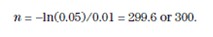
For example, if the actual defect rate were 1% (_p_ = 0.01), meaning that 1% of the finished packages contained at least one piece of the screen, and 100 samples were taken, then _np_ = 1 and _P_ = 0.368. This is the chance the batch would be incorrectly released to the marketplace.
You might not be comfortable with that high of a risk. If, instead of 0.368, you wanted to fix the risk at a small number such as 0.05, then you can calculate the corresponding sample size by solving the previous equation for _n_:
Then substitute 0.05, the risk, for _P_. If the actual defect rate were 1%, the sample size required to detect it with only a 5% chance of error is
As you can see, the choice of sample size depends on the risk of accepting, or releasing to the marketplace, a defective rate of a certain proportion. How are those numbers chosen? They depend on the associated costs and risks.
What is the cost—in terms of negative publicity and consumer alienation—of releasing defective product to the market? Are there health and safety concerns? Conversely, what is the cost of destroying the batch of product? The decision of sample size is not a statistical one, but rather one of choice underpinned by the statistical model.
It can be helpful to display multiple choices so the decision maker can examine the pros and cons of alternative sampling plans. This can be done through the use of curves that show, for fixed risk (_P_), the sample sizes corresponding to hypothetical true defect rates. Sample sizes grow rapidly as the desired proportion defective to be detected decreases. The curves in Figure 1 relate to the situation in which no defective units are permitted for batch acceptance. Similar curves can be drawn for plans corresponding to other acceptance numbers.
http://www.asq.org/img/qp/100936-figure1.gif
Gooey raisins
A process engineer was given responsibility to devise a method of depositing a sugar slurry containing raisins on a breakfast confection. The number of raisins was low relative to the mass of the entire slurry.
The specific gravity of the slurry matched that of the raisins as closely as he could get it, so he was dismayed when the depositor failed to place exactly two raisins on each confection. His conclusion was lack of thorough mixing. Yet, repeated efforts to improve the mixing process failed.
What was going wrong? The Poisson distribution comes to the rescue. Suppose the number of raisins in the slurry tank is such that, on average, he might expect two raisins on each confection. What distribution of raisins might he expect to see due to chance variation?
Recall the Poisson density function:
Here, we have l, the expected mean, equal to two raisins per confection. If you want to know what percentage of confections will have exactly two raisins (_x_ = 2) under perfect mixing, calculate:
This means that about 27.1% of the confections will have exactly two raisins deposited on them.
Table 1 shows the full distribution of raisins under perfect mixing. Notice there will be as many confections with one raisin as there are with two (27.1% each No raisins will appear at all in 13.5% of the confections, and about one-third of the confections will have more than two raisins. Almost 5% will have five or six raisins, and confections with seven or more raisins will be very rare.
http://www.asq.org/img/qp/100936-table1.gif
The conclusion? If marketplace viability depends on having exactly two raisins per confection, a different process will be needed, so you better rig a device that places raisins separately from the slurry.
If you have gotten this far, thanks. Right now, you are probably thinking about situations in which you might use the Poisson distribution or you might have if you had only thought if it.
In general, the use of the Poisson distribution for this kind of problem is only valid if the number of incidents (screen pieces in the first example and raisins in the second) is low relative to the overall mass. There are a few other assumptions you can find in your favorite statistics book.
The Poisson model is a useful component in your bag of tricks.
Lynne B. Hare is a statistical consultant. He holds a doctorate in statistics from Rutgers University in New Brunswick, NJ. He is a past chairman of the ASQ Statistics Division and a fellow of ASQ and the American Statistical Association.


你好,我是小编H。请对以下文章有翻译兴趣的组员留下你的预计完成时间,并发短信息联系小编H,以便小编登记翻译者信息以及文章最终完成时的奖惩工作。感谢支持翻译组!
by Lynne B. Hare
The Poisson distribution (pronounced "pwas-son" where the n is spoken through the nose—don’t ask) may be the Rodney Dangerfield of statistics. It doesn’t get the use—and respect—it deserves. Yet, when applied properly, it can aid the decision-making process considerably.
Here are two examples of its application in the real world. Given these, perhaps you can think of more applications in your own line of work.
Needles in haystacks
For want of preventive maintenance, a screen broke off its frame, disintegrated, mixed with a key product ingredient and then mixed with the finished product. "We think we got it all," said the quality manager. "We ran the finished product over magnets, and we’ve captured enough pieces to reproduce almost an entire screen. Now, we want to sample to make sure we got it all. How many samples do we need if we want to be 100% certain?"
Well, if love means never having to say you’re sorry, statistics means never having to say you’re certain—there’s no such thing as 100% certainty, but you can get close.
Suppose the finished product mass is divided into customer offering quantities, and there are many of these in the offending batch. Define a defective unit as a package containing one or more pieces of screen. If a defective unit is found during sampling, you would conclude the magnets were not completely effective. How many samples must you take to be persuaded the magnets were effective?
A useful model to answer this question is the Poisson distribution. Formally, it is:
in which _e_ is the base of the natural logarithm (e = 2.718), λ is the distribution mean or expected value (typically estimated by the product of _n_, the number of samples, and _p_, the estimate of the proportion defective), and _x_ is the number of screen pieces found.
Because you would conclude the magnets were not fully effective if you found one defective unit, _x_ in the earlier model is set to zero, and the equation reduces to:
in which _P_ is the probability you would accept or release the product to the marketplace.
For example, if the actual defect rate were 1% (_p_ = 0.01), meaning that 1% of the finished packages contained at least one piece of the screen, and 100 samples were taken, then _np_ = 1 and _P_ = 0.368. This is the chance the batch would be incorrectly released to the marketplace.
You might not be comfortable with that high of a risk. If, instead of 0.368, you wanted to fix the risk at a small number such as 0.05, then you can calculate the corresponding sample size by solving the previous equation for _n_:
Then substitute 0.05, the risk, for _P_. If the actual defect rate were 1%, the sample size required to detect it with only a 5% chance of error is
As you can see, the choice of sample size depends on the risk of accepting, or releasing to the marketplace, a defective rate of a certain proportion. How are those numbers chosen? They depend on the associated costs and risks.
What is the cost—in terms of negative publicity and consumer alienation—of releasing defective product to the market? Are there health and safety concerns? Conversely, what is the cost of destroying the batch of product? The decision of sample size is not a statistical one, but rather one of choice underpinned by the statistical model.
It can be helpful to display multiple choices so the decision maker can examine the pros and cons of alternative sampling plans. This can be done through the use of curves that show, for fixed risk (_P_), the sample sizes corresponding to hypothetical true defect rates. Sample sizes grow rapidly as the desired proportion defective to be detected decreases. The curves in Figure 1 relate to the situation in which no defective units are permitted for batch acceptance. Similar curves can be drawn for plans corresponding to other acceptance numbers.
http://www.asq.org/img/qp/100936-figure1.gif
Gooey raisins
A process engineer was given responsibility to devise a method of depositing a sugar slurry containing raisins on a breakfast confection. The number of raisins was low relative to the mass of the entire slurry.
The specific gravity of the slurry matched that of the raisins as closely as he could get it, so he was dismayed when the depositor failed to place exactly two raisins on each confection. His conclusion was lack of thorough mixing. Yet, repeated efforts to improve the mixing process failed.
What was going wrong? The Poisson distribution comes to the rescue. Suppose the number of raisins in the slurry tank is such that, on average, he might expect two raisins on each confection. What distribution of raisins might he expect to see due to chance variation?
Recall the Poisson density function:
Here, we have l, the expected mean, equal to two raisins per confection. If you want to know what percentage of confections will have exactly two raisins (_x_ = 2) under perfect mixing, calculate:
This means that about 27.1% of the confections will have exactly two raisins deposited on them.
Table 1 shows the full distribution of raisins under perfect mixing. Notice there will be as many confections with one raisin as there are with two (27.1% each No raisins will appear at all in 13.5% of the confections, and about one-third of the confections will have more than two raisins. Almost 5% will have five or six raisins, and confections with seven or more raisins will be very rare.
http://www.asq.org/img/qp/100936-table1.gif
The conclusion? If marketplace viability depends on having exactly two raisins per confection, a different process will be needed, so you better rig a device that places raisins separately from the slurry.
If you have gotten this far, thanks. Right now, you are probably thinking about situations in which you might use the Poisson distribution or you might have if you had only thought if it.
In general, the use of the Poisson distribution for this kind of problem is only valid if the number of incidents (screen pieces in the first example and raisins in the second) is low relative to the overall mass. There are a few other assumptions you can find in your favorite statistics book.
The Poisson model is a useful component in your bag of tricks.
Lynne B. Hare is a statistical consultant. He holds a doctorate in statistics from Rutgers University in New Brunswick, NJ. He is a past chairman of the ASQ Statistics Division and a fellow of ASQ and the American Statistical Association.
没有找到相关结果
已邀请:


3 个回复
小编H (威望:4) (广东 广州) 互联网 员工
赞同来自: